I’m trying to build a age-period-cohort model of smoking using the various MPC cleaned datasets. Since I have the most experience with BRFSS, I started with just some simple visualizations looking at the data through a cohort lense. Things run a bit slow to use srvyr or survey functions to get estimates of variance, so I’ll just use weighted means and rely on inter-year variability to show the variation (at least for now, for this exploratory work).
I think the best graphs come from the most simple variable whether the
respondent has smoked 100 cigarettes total in their lifetime. Here they
are in gif form:
If that gif makes your head swim, here’s a faceted graph showing every 5th cohort’s trends.
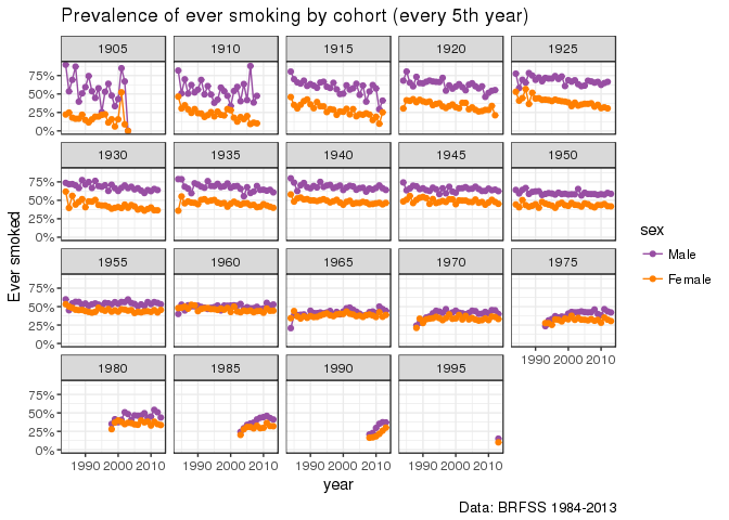
I see 4 phases of broad trends:
-
Not enough data (Roughly 1890-1905)
At first there’s just not enough data and so there’s too much variation to see any clear trends. BRFSS doesn’t have a lot of people in the older age groups. A big part of this is due to people dying, but also the BRFSS sample frame doesn’t cover nursing homes or long-term care facilities so it’s coverage of older respondents is pretty poor. Further, to make this anaysis as simple as possible, I don’t include respondents in the top-coded age categories (97 in 1984, 80 in 2012 and later, and 99 in all other years). -
Differential mortality & women catch up (Roughly 1905-1935)
Because we are looking at ever smoking, the fact that the slope goes down is somewhat confusing. For each person, they can never change from an ever smoker to a never smoker. Yet, the percentage of the cohort who are ever smokers goes down in this period. This is self-reported data of course, so some of it could be changes in recall or social desirability bias as time goes on, but a big part of it is likely due to the fact that there is differential mortality between people who have ever smoked and those who have not. This can be caused both by the harmful effects of smoking as well as other behaviors that are correlated with smoking such as alcohol and other drugs and other risk behaviors.Another interesting thing to look at in this phase of the gif is that women are catching up to men in smoking prevalence. Presumably this is evidence of women’s liberation and other changes in social norms around women’s behavior.
-
Rates fall, and men converge to women (Roughly 1935-1965)
After generally increasing (probably partly due to differential mortality), the rates begin to fall pretty quickly cohort birth year over year. At the beginning of this phase, ~75% of men and 60% of women have ever smoked, and by the end they are below 50%. -
Seeing introduction of smoking (1965-2013) These groups are the first that we are seeing young enough for significant numbers of new ever smokers to be introduced (both because they are younger when the first survey interviewed them and because the age of smoking introduction is getting older). This is shown by the upward trend for each cohort. It appears like men are starting to smoke more than women again, though there’s not enough data to be completely sure.
Those are the first set of graphs I made from BRFSS. Hopefully soon I’ll show something about currently smoking and retrospective prevalence from BRFSS as well as some of the other surveys we have harmonized (YRBSS, NSDUH, NHIS).
I can’t really share the data yet (hopefully soon), but here’s the code used to produce these plots (man it’d be nice to have collapsible code blocks in this blog CMS).
suppressPackageStartupMessages({
  library(dplyr)
  library(gganimate) # requires devtools::install_github("gergness/gganimate@1d611fa")
  library(ggplot2)
  library(mpctools)
  library(purrr)
  library(readr)
  library(srvyr)
  library(tibble)
  library(tidyr)
})

# Load data ---------
out_dir <- "~/smoking_age_cohort/interim_data/"
brfss_years <- 1984:2013

calc_age_clean <- function(age, year) {
  # NAs for top code because we don't know their real age...
  ifelse((year == 1984 & age >= 97) |
           (year >= 1985 & year <= 2012 & age >= 99) |
           (year == 2013 & age >= 80),
         NA, age)

}

all_brfss <- map_df(brfss_years, function(yyy) {
  out <- readRDS(paste0(out_dir, "/person/brfss", yyy, "a.Rds")) %>%
    set_names(tolower(names(.))) %>%
    mutate(
      age = as.numeric(age),
      age_clean = calc_age_clean(age, yyy),
      cohort = yyy - age_clean,
      sex = haven::as_factor(sex),
      survey_year = yyy
    ) %>%
    filter(!is.na(age_clean))

  # Get weights
  if (yyy <= 2010) {
    out <- mutate(out, weights = landwt)
  } else {
    out <-  mutate(out, weights = llcpwt)
  }

  out
})


# Calcualte ever Smoked -------------
calc_smokev_bin <- function(smokev) {
  smokev == 2
}

ever_smoked_data <- all_brfss %>%
  mutate(
    smokev_bin = calc_smokev_bin(smokev),
    year = survey_year
  ) %>%
  group_by(sex, age_clean, cohort, year) %>%
  summarize(
    ever_smoked = weighted.mean(smokev_bin, weights, na.rm = TRUE),
    n = sum(!is.na(smokev_bin))
  )

# Animated plot ------------
ever_smoked_plot_data <- ever_smoked_data %>%
  # To make graphs more readable
  filter(cohort > 1905)
plot <- ggplot(
  ever_smoked_plot_data,
  aes(x = year, y = ever_smoked, group = paste0(sex, "-", cohort), color = sex,
      frame = cohort, cumulative = TRUE, alpha_decay = function(x) exp(-x/5))
) +
  geom_line() +
  geom_point() +
  theme_bw() +
  scale_color_manual(values = c("#984ea3", "#ff7f00")) +
  scale_y_continuous("Ever smoked", labels = scales::percent) +
  labs(
    title = "Cohort: ",
    subtitle = "Prevalence of ever smoking",
    caption = "Data: BRFSS 1984-2013"
  )

gg_animate(plot, interval = 0.15)

# Static plot ------------
ever_smoked_plot_data <- ever_smoked_data %>%
  # To make graphs more readable
  filter(cohort %in% seq(1905, 2005, by = 5))

ggplot(ever_smoked_plot_data, aes(x = year, y = ever_smoked, group = sex, color = sex)) +
  geom_line() +
  geom_point() +
  facet_wrap(~cohort) +
  theme_bw() +
  scale_color_manual(values = c("#984ea3", "#ff7f00")) +
  scale_y_continuous("Ever smoked", labels = scales::percent) +
  labs(
    title = "Prevalence of ever smoking by cohort (every 5th year)",
    caption = "Data: BRFSS 1984-2013"
  )