`srvyr` compared to the `survey` package
Greg Freedman
2024-10-29
Source:vignettes/srvyr-vs-survey.Rmd
srvyr-vs-survey.RmdThe srvyr package adds dplyr like syntax to
the survey package. This vignette focuses on how
srvyr compares to the survey package, for more
information about survey design and analysis, check out the vignettes in
the survey package, or Thomas Lumley’s book, Complex
Surveys: A Guide to Analysis Using R. (Also see the bottom of
this document for some more resources).
Everything that srvyr can do, can also be done in
survey. In fact, behind the scenes the survey
package is doing all of the hard work for srvyr.
srvyr strives to make your code simpler and more easily
readable to you, especially if you are already used to the
dplyr package.
Motivating example
The dplyr package has made it easy to write code to
summarize data. For example, if we wanted to check how the year-to-year
change in academic progress indicator score varied by school level and
percent of parents were high school graduates, we can do this:
library(survey)
library(ggplot2)
library(dplyr)

data(api)

out <- apistrat %>%
  mutate(hs_grad_pct = cut(hsg, c(0, 20, 100), include.lowest = TRUE,
                           labels = c("<20%", "20+%"))) %>%
  group_by(stype, hs_grad_pct) %>%
  summarize(api_diff = weighted.mean(api00 - api99, pw),
            n = n())

ggplot(data = out, aes(x = stype, y = api_diff, group = hs_grad_pct, fill = hs_grad_pct)) +
  geom_col(stat = "identity", position = "dodge") +
  geom_text(aes(y = 0, label = n), position = position_dodge(width = 0.9), vjust = -1)
## Warning in geom_col(stat = "identity", position = "dodge"): Ignoring
## unknown parameters: `stat`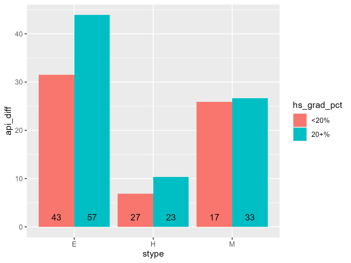
However, if we wanted to add error bars to the graph to capture the
uncertainty due to sampling variation, we have to completely rewrite the
dplyr code for the survey package.
srvyr allows a more direct translation.
Preparing a survey dataset
as_survey_design(), as_survey_rep() and
as_survey_twophase() are analogous to
survey::svydesign(), survey::svrepdesign() and
survey::twophase() respectively. Because they are designed
to match dplyr’s style of non-standard evaluation, they
accept bare column names instead of formulas (~). They also move the
data argument first, so that it is easier to use magrittr
pipes (%>%).
library(srvyr)

# simple random sample
srs_design_srvyr <- apisrs %>% as_survey_design(ids = 1, fpc = fpc)

srs_design_survey <- svydesign(ids = ~1, fpc = ~fpc, data = apisrs)
The srvyr functions also accept
dplyr::select()’s special selection functions (such as
starts_with(), one_of(), etc.), so these
functions are analogous:
# selecting variables to keep in the survey object (stratified example)
strat_design_srvyr <- apistrat %>%
  as_survey_design(1, strata = stype, fpc = fpc, weight = pw,
                variables = c(stype, starts_with("api")))

strat_design_survey <- svydesign(~1, strata = ~stype, fpc = ~fpc,
                                 variables = ~stype + api99 + api00 + api.stu,
                                 weight = ~pw, data = apistrat)
The function as_survey() will automatically choose
between the three as_survey_* functions based on the
arguments, so you can save a few keystrokes.
Data manipulation
Once you’ve set up your survey data, you can use dplyr
verbs such as mutate(), select(),
filter() and rename().
strat_design_srvyr <- strat_design_srvyr %>%
  mutate(api_diff = api00 - api99) %>%
  rename(api_students = api.stu)

strat_design_survey$variables$api_diff <- strat_design_survey$variables$api00 -
  strat_design_survey$variables$api99
names(strat_design_survey$variables)[names(strat_design_survey$variables) == "api.stu"] <- "api_students"
Note that arrange() is not available, because the
srvyr object expects to stay in the same order. Nor are
two-table verbs such as full_join(),
bind_rows(), etc. available to srvyr objects
either because they may have implications on the survey design. If you
need to use these functions, you should use them earlier in your
analysis pipeline, when the objects are still stored as
data.frames.
Summary statistics
Of the entire population
srvyr also provides summarize() and several
survey-specific functions that calculate summary statistics on numeric
variables: survey_mean(), survey_total(),
survey_quantile() and survey_ratio(). These
functions differ from their counterparts in survey because
they always return a data.frame in a consistent format. As such, they do
not return the variance-covariance matrix, and so are not as
flexible.
# Using srvyr
out <- strat_design_srvyr %>%
  summarize(api_diff = survey_mean(api_diff, vartype = "ci"))

out
## # A tibble: 1 × 3
## api_diff api_diff_low api_diff_upp
## <dbl> <dbl> <dbl>
## 1 32.9 28.8 36.9
# Using survey
out <- svymean(~api_diff, strat_design_survey)

out
## mean SE
## api_diff 32.893 2.0511
confint(out)## 2.5 % 97.5 %
## api_diff 28.87241 36.91262By group
srvyr also allows you to calculate statistics on numeric
variables by group, using group_by().
# Using srvyr
strat_design_srvyr %>%
  group_by(stype) %>%
  summarize(api_increase = survey_total(api_diff >= 0),
            api_decrease = survey_total(api_diff < 0))
## # A tibble: 3 × 5
## stype api_increase api_increase_se api_decrease api_decrease_se
## <fct> <dbl> <dbl> <dbl> <dbl>
## 1 E 4067. 119. 354. 119.
## 2 H 498. 49.4 257. 49.4
## 3 M 998. 19.9 20.4 19.9
# Using survey
svyby(~api_diff >= 0, ~stype, strat_design_survey, svytotal)
## stype api_diff >= 0FALSE api_diff >= 0TRUE se.api_diff >= 0FALSE
## E E 353.68 4067.32 119.17185
## H H 256.70 498.30 49.37208
## M M 20.36 997.64 19.85371
## se.api_diff >= 0TRUE
## E 119.17185
## H 49.37208
## M 19.85371Proportions by group
You can also calculate the proportion or count in each group of a
factor or character variable by leaving x empty in
survey_mean() or survey_total().
# Using srvyr
srs_design_srvyr %>%
  group_by(awards) %>%
  summarize(proportion = survey_mean(),
            total = survey_total())
## # A tibble: 2 × 5
## awards proportion proportion_se total total_se
## <fct> <dbl> <dbl> <dbl> <dbl>
## 1 No 0.38 0.0338 2354. 210.
## 2 Yes 0.62 0.0338 3840. 210.
# Using survey
svymean(~awards, srs_design_survey)
## mean SE
## awardsNo 0.38 0.0338
## awardsYes 0.62 0.0338
svytotal(~awards, srs_design_survey)## total SE
## awardsNo 2353.7 209.65
## awardsYes 3840.3 209.65Unweighted calculations
Finally, the unweighted() function can act as an escape
hatch to calculate unweighted calculations on the dataset.
## # A tibble: 3 × 2
##   stype     n
##   <fct> <int>
## 1 E       100
## 2 H        50
## 3 M        50
# Using survey
svyby(~api99, ~stype, strat_design_survey, unwtd.count)
## stype counts se
## E E 100 0
## H H 50 0
## M M 50 0Back to the example
So now, we have all the tools needed to create the first graph and
add error bounds. Notice that the data manipulation code is nearly
identical to the dplyr code, with a little extra set up,
and replacing weighted.mean() with
survey_mean.
strat_design <- apistrat %>%
  as_survey_design(strata = stype, fpc = fpc, weight  = pw)

out <- strat_design %>%
  mutate(hs_grad_pct = cut(hsg, c(0, 20, 100), include.lowest = TRUE,
                           labels = c("<20%", "20+%"))) %>%
  group_by(stype, hs_grad_pct) %>%
  summarize(api_diff = survey_mean(api00 - api99, vartype = "ci"),
            n = unweighted(n()))

ggplot(data = out, aes(x = stype, y = api_diff, group = hs_grad_pct, fill = hs_grad_pct,
                       ymax = api_diff_upp, ymin = api_diff_low)) +
  geom_col(stat = "identity", position = "dodge") +
  geom_errorbar(position = position_dodge(width = 0.9), width = 0.1) +
  geom_text(aes(y = 0, label = n), position = position_dodge(width = 0.9), vjust = -1)
## Warning in geom_col(stat = "identity", position = "dodge"): Ignoring
## unknown parameters: `stat`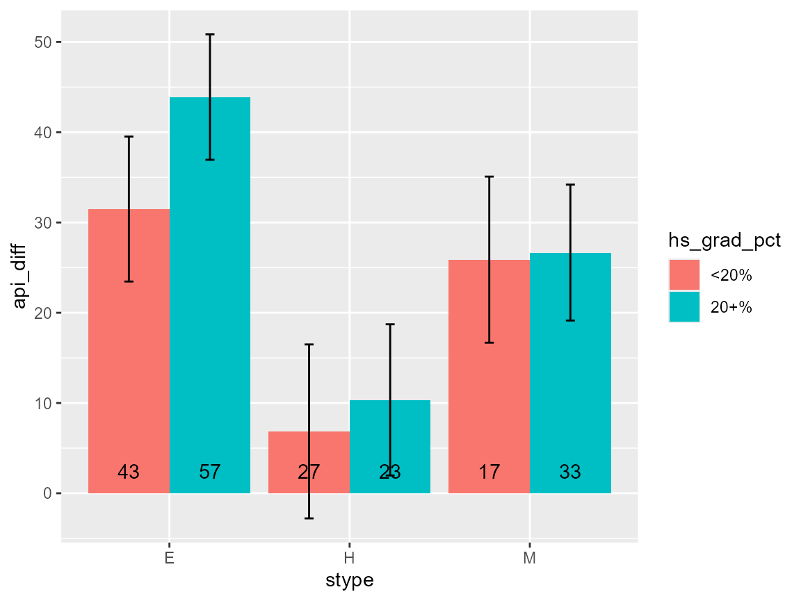
Comparison to the survey package (Degrees of freedom)
For the most part, srvyr tries to be a drop-in
replacement for the survey package, only changing the syntax that you
wrote. However, the way that calculations of degrees of freedom when
calculating confidence intervals is different.
srvyr assumes that you want to use the true degrees of
freedom by default, but the survey package uses
Inf as the default. You can use the argument
df to get the same result as the survey package.
# Set pillar print methods so tibble has more decimal places
old_sigfig <- options("pillar.sigfig")
options("pillar.sigfig" = 5)

# survey default
estimate <- svymean(~api99, strat_design)
confint(estimate)
## 2.5 % 97.5 %
## api99 609.8659 648.9238
# srvyr default
strat_design %>%
  summarize(x = survey_mean(api99, vartype = "ci"))
## # A tibble: 1 × 3
## x x_low x_upp
## <dbl> <dbl> <dbl>
## 1 629.39 609.75 649.04
# setting the degrees of freedom so srvyr matches survey default
strat_design %>%
  summarize(x = survey_mean(api99, vartype = "ci", df = Inf)) %>%
  print()
## # A tibble: 1 × 3
## x x_low x_upp
## <dbl> <dbl> <dbl>
## 1 629.39 609.87 648.92
# setting the degrees of freedom so survey matches survey default
confint(estimate, df = degf(strat_design))
## 2.5 % 97.5 %
## api99 609.7452 649.0445
# reset significant figures
options("pillar.sigfig" = old_sigfig)
Grab Bag
Using survey functions on srvyr
objects
Because srvyr objects are just survey
objects with some extra structure, all of the functions from
survey will still work with them. If you need to calculate
something beyond simple summary statistics, you can use
survey functions.
##
## Call:
## svyglm(formula = api00 ~ ell + meals + mobility, design = strat_design)
##
## Survey design:
## Called via srvyr
##
## Coefficients:
##             Estimate Std. Error t value Pr(>|t|)
## (Intercept) 820.8873    10.0777  81.456   <2e-16 ***
## ell          -0.4806     0.3920  -1.226    0.222
## meals        -3.1415     0.2839 -11.064   <2e-16 ***
## mobility      0.2257     0.3932   0.574    0.567
## ---
## Signif. codes:  0 '***' 0.001 '**' 0.01 '*' 0.05 '.' 0.1 ' ' 1
##
## (Dispersion parameter for gaussian family taken to be 5171.966)
##
## Number of Fisher Scoring iterations: 2
Using expressions to create variables on the fly
Like dplyr, srvyr allows you to use
expressions in the arguments, allowing you to create variables in a
single step. For example, you can use expressions:
- as the arguments inside the survey statistic functions like
survey_mean
strat_design %>%
  summarize(prop_api99_over_700 = survey_mean(api99 > 700))
## # A tibble: 1 × 2
## prop_api99_over_700 prop_api99_over_700_se
## <dbl> <dbl>
## 1 0.306 0.0356- as an argument to
summarize
strat_design %>%
  group_by(awards) %>%
  summarize(percentage = 100 * survey_mean())
## # A tibble: 2 × 3
## awards percentage percentage_se
## <fct> <dbl> <dbl>
## 1 No 36.1 3.44
## 2 Yes 63.9 3.44- and you can even create variables inside of
group_by
strat_design %>%
  group_by(api99_above_700 = api99 > 700) %>%
  summarize(api00_mn = survey_mean(api00))
## # A tibble: 2 × 3
## api99_above_700 api00_mn api00_mn_se
## <lgl> <dbl> <dbl>
## 1 FALSE 599. 7.88
## 2 TRUE 805. 7.15Though on-the-fly expressions are syntactically valid, it is possible to make statistically invalid numbers from them. For example, though the standard error and confidence intervals can be multiplied by a scalar (like 100), the variance does not scale the same way, so the following is invalid:
# BAD DON'T DO THIS!
strat_design %>%
  group_by(awards) %>%
  summarize(percentage = 100 * survey_mean(vartype = "var"))
# VARIANCE IS WRONG
Non-Standard evaluation
Srvyr supports the non-standard evaluation conventions that dplyr
uses. If you’d like to use a function programmatically, you can use the
functions from rlang like the {{ operator (aka “curly
curly”) from rlang.
Here’s a quick example, but please see the dplyr vignette vignette("programming", package = "dplyr")
for more details.
mean_with_ci <- function(.data, var) {
  summarize(.data, mean = survey_mean({{var}}, vartype = "ci"))
}

srs_design_srvyr <- apisrs %>% as_survey_design(fpc = fpc)

mean_with_ci(srs_design_srvyr, api99)
## # A tibble: 1 × 3
## mean mean_low mean_upp
## <dbl> <dbl> <dbl>
## 1 625. 606. 643.Srvyr will also follow dplyr’s lead on deprecating the old methods of
NSE, such as rlang::quo, and !!, in addition
to the so-called “underscore functions” (like summarize_).
Currently, they have been soft-deprecated, they may be removed
altogether in some future version of srvyr.
Working column-wise
As of version 1.0 of srvyr, it supports dplyr’s across function, so
when you want to calculate a statistic on more than one variable, it is
easy to do so. See vignette("colwise", package = "dplyr")
for more details, but here is another quick example:
# Calculate survey mean for all variables that have names starting with "api"
strat_design %>%
  summarize(across(starts_with("api"), survey_mean))
## # A tibble: 1 × 6
## api00 api00_se api99 api99_se api.stu api.stu_se
## <dbl> <dbl> <dbl> <dbl> <dbl> <dbl>
## 1 662. 9.41 629. 9.96 498. 16.1Srvyr also supports older methods of working column-wise, the “scoped
variants”, such as summarize_at, summarize_if,
summarize_all and summarize_each. Again, these
are maintained for backwards compatibility, matching what the tidyverse
team has done, but may be removed from a future version.
Calculating proportions in groups
You can calculate the weighted proportion that falls into a group
using the survey_prop() function (or the
survey_mean() function with no x argument).
The proportion is calculated by “unpeeling” the last variable used in
group_by() and then calculating the proportion within the
other groups that fall into the last group (so that the proportion
within each group that was unpeeled sums to 100%).
# Calculate the proportion that falls into each category of `awards` per `stype`
strat_design %>%
  group_by(stype, awards) %>%
  summarize(prop = survey_prop())
## When `proportion` is unspecified, `survey_prop()` now defaults to `proportion = TRUE`.
## ℹ This should improve confidence interval coverage.
## This message is displayed once per session.## # A tibble: 6 × 4
## # Groups: stype [3]
## stype awards prop prop_se
## <fct> <fct> <dbl> <dbl>
## 1 E No 0.270 0.0441
## 2 E Yes 0.730 0.0441
## 3 H No 0.680 0.0644
## 4 H Yes 0.320 0.0644
## 5 M No 0.520 0.0696
## 6 M Yes 0.480 0.0696If you want to calculate the proportion for groups from multiple
variables at the same time that add up to 100%, the
interact function can help. The interact
function creates a variable that is automatically split apart so that
more than one variable can be unpeeled.
# Calculate the proportion that falls into each category of both `awards` and `stype`
strat_design %>%
  group_by(interact(stype, awards)) %>%
  summarize(prop = survey_prop())
## # A tibble: 6 × 4
## stype awards prop prop_se
## <fct> <fct> <dbl> <dbl>
## 1 E No 0.193 0.0315
## 2 E Yes 0.521 0.0315
## 3 H No 0.0829 0.00785
## 4 H Yes 0.0390 0.00785
## 5 M No 0.0855 0.0114
## 6 M Yes 0.0789 0.0114Learning More
Here are some free resources put together by the community about srvyr:
-
“How-to”s & examples of using srvyr
- Stephanie Zimmer, Rebecca Powell and Isabella Velásquez’s book Exploring Complex Survey Data Analysis Using R (releasing in November 2024). See also their 2021 AAPOR Workshop “Tidy Survey Analysis in R using the srvyr Package”
- “The Epidemiologist R Handbook”, by Neale Batra et al. has a chapter on survey analysis with srvyr and survey package examples
- Kieran Healy’s book “Data Visualization: A Practical Introduction” has a section on using srvyr to visualize the ESS.
- The IPUMS PMA team’s blog had a series showing examples of using the PMA COVID survey panel with weights
- “Open Case Studies: Vaping Behaviors in American Youth” by Carrie Wright, Michael Ontiveros, Leah Jager, Margaret Taub, and Stephanie Hicks is a detailed case study that includes using srvyr to analyze the National Youth Tobacco Survey.
- “How to plot Likert scales with a weighted survey in a dplyr friendly way” by Francisco Suárez Salas
- The tidycensus package vignette “Working with Census microdata” includes information about using the weights from the ACS retrieved from the census API.
- “The Joy of Calculating the Direct Standard Error for PUMS Estimates” by GitHub user @ldaly
-
About survey statistics
- Thomas Lumley’s book “Complex Surveys: a guide to analysis using R”
- Chris Skinner. Jon Wakefield. “Introduction to the Design and Analysis of Complex Survey Data.” Statist. Sci. 32 (2) 165 - 175, May 2017. 10.1214/17-STS614
- Sharon Lohr’s textbook “Sampling: Design and Analysis”. Second or Third Editions
- “Survey weighting is a mess” is the opening to Andrew Gelman’s “Struggles with Survey Weighting and Regression Modeling”
- Anthony Damico’s website “Analyze Survey Data for Free” has the weight specifications for a wide variety of public use survey datasets.
-
Working programmatically and/or on multiple columns at once
(eg
dplyr::acrossandrlang’s “curly curly”{{}})- dplyr’s included package vignettes “Column-wise operations” & “Programming with dplyr”
-
Non-English resources
- Em português: “Análise de Dados Amostrais Complexos” by Djalma Pessoa and Pedro Nascimento Silva
- En español: “Usando R para jugar con los microdatos del INEGI” by Claudio Daniel Pacheco Castro
- Tiếng Việt: “Dịch tễ học ứng dụng và y tế công cộng với R”
- På norsk: Data med vekter i R by Øyvind Bugge Solheim
-
Other cool stuff that uses srvyr
- A (free) graphical interface allowing exploratory data analysis of survey data without writing code: iNZight (and survey data instructions)
- “serosurvey: Serological Survey Analysis For Prevalence Estimation Under Misclassification” by Andree Valle Campos
- Several packages on CRAN depend on srvyr, you can see them by looking at the reverse Imports/Suggestions on CRAN.
Still need help?
I think the best way to get help is to form a specific question and ask it in some place like posit’s community website (known for it’s friendly community) or stackoverflow.com (maybe not known for being quite as friendly, but probably has more people). If you think you’ve found a bug in srvyr’s code, please file an issue on GitHub, but note that I’m not a great resource for helping specific issue, both because I have limited capacity but also because I do not consider myself an expert in the statistical methods behind survey analysis.
Have something to add?
These resources were mostly found via vanity searches on twitter & github. If you know of anything I missed, or have written something yourself, please let me know in this GitHub issue!